



















Image and text models moved to deep learning years ago. Structured tables stayed with gradient-boosted trees, and libraries such as XGBoost and CatBoost remained the strongest choice for prediction tasks on rows and columns.
That position has shifted in the past two years. A model published in Nature in January 2025 reached higher accuracy in 2.8 seconds than an ensemble of tuned baselines reached in four hours. Its pretraining used only synthetic tables, which is the part of the result that explains the speed.
This article explains what a tabular foundation model is and how TabPFN produces predictions without fitting to your dataset. It then covers what the published benchmarks report and where gradient boosting still wins.
Why Structured Data Resisted Deep Learning
Structured data resisted deep learning because of the way a table is shaped. On images and text, neural networks exploit structure that the format itself supplies, since pixels near each other relate to each other and words follow a sequence.
A table carries no comparable structure, and three properties explain why.
- Columns are heterogeneous. One column records revenue as a dollar amount while the next stores a product category as text. A third carries a single binary flag. Each column carries its own meaning and its own scale, and nothing connects column three to column four the way one pixel connects to its neighbor.
- Column order carries no information. Shuffle the columns of a spreadsheet and the data means exactly what it meant before. Shuffle the pixels of a photograph and the image is destroyed.
- Business tables are small. A churn dataset of 40,000 rows supplies a fraction of what a neural network needs. Language models train on trillions of tokens, and that gap removes the main advantage neural networks hold.
Decision trees handle all three properties natively. A tree splits on one feature at a time, which accommodates mixed types and mixed scales directly. Gradient boosting then extracts usable accuracy from a few thousand rows, and that pairing was the standard approach for more than a decade.
What Is a Tabular Foundation Model?
A tabular foundation model is a single pretrained model that makes predictions on a new table without being trained on that table. You pass your labeled rows to the model at prediction time, and it returns predictions for the rows you want scored.
The conventional workflow asks more of you at every stage. You choose an algorithm and select hyperparameters, then fit the model to your training rows. You repeat that cycle until the validation score stops improving, and the result is a model that exists only for that dataset.
A tabular foundation model arrives already trained. Your data enters a system whose parameters were fixed before you opened your file.
| Stage | Conventional Pipeline | Tabular Foundation Model |
|---|---|---|
| What you fit | A new model for each dataset | Nothing, since the model is already trained |
| Where your data enters | Training | Prediction time, supplied as context |
| Time to a usable result | Hours of tuning | Seconds |
| What the model learned from | Your rows | Synthetic tables |
| Cost per prediction | Low | Higher |
| Dataset size it suits | Whatever you can afford to train on | Bounded by what the model can hold |
Speed and serving cost share one cause. Skipping training delivers the first result in seconds, and running a full forward pass for every prediction raises the cost of each one. Your decision needs both numbers.
The term foundation model carries the same meaning here that it carries for language. One expensive pretraining run produces a general-purpose system, and downstream users apply it to their own problems without repeating that run. What changes in the tabular case is the pretraining material, since the tables behind TabPFN were produced by simulation.
How TabPFN Learns Without Seeing Your Data
All of TabPFN's learning happened before your dataset existed, in a single pretraining stage built entirely from simulated data. The model's parameters stay frozen through every prediction it makes. The three mechanisms below explain how that pretraining transfers to your table.
- A synthetic prior. The model was pretrained on roughly 130 million synthetic tables, generated from structural causal models. A structural causal model is a small simulated system in which some variables influence others through defined relationships. The generated tables vary in structure and feature type, with missing values and noise introduced deliberately.
- In-context learning. TabPFN receives your labeled training rows and your unlabeled test rows together, then predicts in a single forward pass. No gradient updates happen for your dataset, which is why the method finishes in seconds.
- Attention across cells. Each table cell gets its own representation. Attention runs across features within a row, then across samples within a column. Predictions therefore stay the same when you reorder your rows or your columns.
TabPFN has therefore already learned the shapes that prediction problems take, and it applies that knowledge to the specific table you supply.
The authors frame the point in Bayesian terms, describing the system as one that "can be viewed as approximating Bayesian prediction for a prior defined by the synthetic datasets." The synthetic tables set out what a dataset is expected to resemble, and your rows indicate which of those expectations apply.
What the Benchmarks Show
Nature's headline result is a timing comparison. "In 2.8 s, TabPFN outperforms an ensemble of the strongest baselines tuned for 4 h in a classification setting." The reported speedup reaches 5,140 times for classification and 3,000 times for regression.
Both accuracy metrics below are normalized so that higher scores indicate better results. On classification, TabPFN reached 0.939 against default CatBoost's 0.752 on ROC AUC, and 0.952 against a tuned CatBoost's 0.822. On regression, TabPFN scored 0.923 on RMSE against the default's 0.872, and 0.968 against the tuned version's 0.875.
Those figures came from datasets of up to 10,000 samples and 500 features, with up to 10 classes.
That ceiling has since risen. The TabPFN-3 technical report, published in May 2026, extends the method to 1 million training rows and 200 features. A single forward pass beat gradient-boosted tree baselines tuned for eight hours, and the system runs up to 20 times faster than the previous release.
On TabArena, a public benchmark for tabular methods, that single pass placed above every other entry including tuned ensembles. A commercial variant that spends extra computation at prediction time matches AutoGluon, an automated machine learning framework, in under a tenth of the runtime.
Where the Model Still Loses
The Nature authors state the limitations directly, and three of them affect how you would deploy the approach.
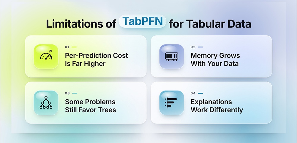
Per-prediction cost is far higher. On a dataset of 10,000 rows and 10 columns, TabPFN needs about 0.2 seconds per sample, or 0.6 seconds without a graphics processing unit. Default CatBoost needs 0.0002 seconds. At high serving volume that gap settles the question on its own, whatever the accuracy comparison shows.
Memory grows with your data. The paper states that memory usage "scales linearly with dataset size, which can be prohibitive for very large datasets." It adds that scaling beyond the tested range "requires further study."
Some problems still favor trees. The authors expect CatBoost and XGBoost to outperform TabPFN on larger datasets, and on highly non-smooth regression tasks. A non-smooth task is one where the relationship between features and target changes sharply across a small input range.
Explanations work differently. A gradient-boosted model yields feature importance from its own trained tree structure. A foundation model keeps its parameters fixed, so you depend on post-hoc methods such as SHAP values, which measure each feature's contribution to a single prediction. The TabPFN-3 report documents caching work that speeds those calculations, and that engineering effort indicates the cost was high enough to matter.
A fourth constraint is commercial. The TabPFN-3 open-source release permits research and internal evaluation, and production deployment requires a separate enterprise license. Resolve that question before advancing from a pilot to production.
How to Test It Against Your Own Baseline
The following steps produce a defensible comparison.
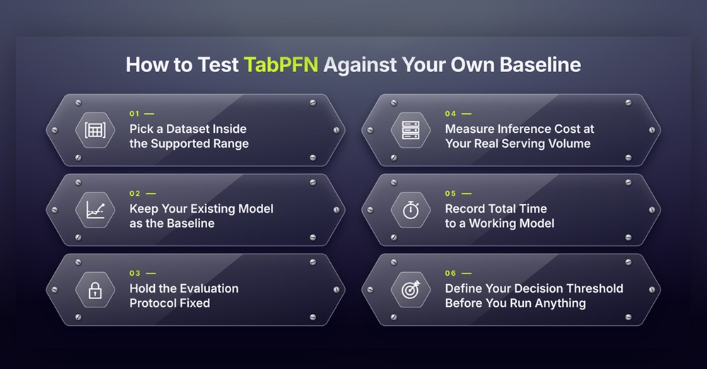
Step 1: Pick a dataset inside the supported range. Match your row count and feature count to the limits of the version you are testing. A dataset outside that range produces a result that tells you nothing about either model.
Step 2: Keep your existing model as the baseline. Your tuned gradient-boosting model is the comparison that matters, since replacing it is the decision in question.
Step 3: Hold the evaluation protocol fixed. Apply identical splits and preprocessing for both candidates, and score them on one metric. This guide to cross-validation and model evaluation covers the methods that give a steady performance estimate across candidate models.
Step 4: Measure inference cost at your real serving volume. Score a batch the size of your production load and record wall-clock time on the hardware you would use in deployment. A per-sample figure from a published benchmark will understate what you face.
Step 5: Record total time to a working model. Include the hours you spend tuning the baseline. Accuracy is one column of your result, and time to a deployable model is the column that justifies a change in workflow.
Step 6: Define your decision threshold before you run anything. Name the accuracy improvement that would justify a switch and the inference latency you can tolerate. A threshold set in advance protects you from reading a small accuracy gain as a reason to rebuild a working pipeline.
Your data preparation stays the same under either approach, and the Python libraries used in modern data engineering handle the loading and shaping work in both cases.
Conclusion
Tabular foundation models shift key prediction work from tuning to pretraining. The tuning cycle that defined structured data modeling for a decade shifts into a pretraining stage someone else already paid for, and your dataset becomes input to a finished model.
The published evidence supports the approach inside its stated range, and the same papers mark the edges of that range in detail. Dataset size and per-prediction cost each decide cases where accuracy alone leaves the question open, and licensing terms can settle the matter before either one applies.
Test one dataset against your current baseline within your next evaluation cycle, holding the evaluation protocol fixed and measuring inference cost at production volume. That single comparison tells you more about where this belongs in your work than any benchmark table can.